XSTARDB
Getting Started
See the installation instructions before using XSTARDB for the first time.
To begin, you must start an ISIS session and load the library:
isis> require( "xstardb" );
Then you must run an XSTAR model with the write_outfile parameter turned on.
The library includes a secondary set of XSTAR model names,
warmabs2 and photemis2,
which contains the additional parameter autoname_outfile.
It doesn't matter which version you use, as long as
write_outfile is enabled. Here is an example model run:
 isis> fit_fun( "powerlaw(1) * warmabs2(1)" );

            isis> set_par( "warmabs2(1).write_outfile", 1 );

            isis> set_par( "warmabs2(1).autoname_outfile", 1 );
The model needs to be evaluated on a wavelength grid.
If you loaded a data set, the grid has already been specified.
If you want to examine simulated spectra, you must create your own grid:
isis> (x1, x2) = linear_grid( 1.0, 40.0, 10000 );
then evaluate it:
isis> y = eval_fun( x1, x2 );
The eval_fun call will cause XSTAR to run a warmabs calculation.
The atomic data will be stored in a file named warmabs_1.fits.
To read in the file:
isis> db = rd_xstar_output( "warmabs_1.fits" );
At this point, the data can be browsed.
We recommend running a search for all XSTAR related commands:
isis> apropos xstar;
Use the help command to view the manual page, for example:
isis> help rd_xstar_output;
A larger set of tutorials utilizing the XSTARDB library will be maintained on github:
https://github.com/eblur/xstardb-tutorials
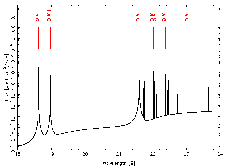
Example 1: A single photemis model
Examine a photemis model where the only heavy metal present is oxygen, in solar abundance (view script).
The basics are covered in this example. The remaining examples on this page omit repeat
commands such as turning on the write_outfile parameter and plotting.
 isis> fit_fun("photemis2(1)");

        isis> set_par("photemis2(1).write_outfile", 1);

        isis> set_par("photemis2(1).autoname_outfile", 1);

        isis> set_par( [3:27], 0 );

        isis> set_par( "photemis2(1).Oabund", 1.0 );

        isis> (x1, x2) = linear_grid( 1.0, 40.0, 10000 );

        isis> y = eval_fun( x1, x2 );

        isis> db = rd_xstar_output( "photemis_1.fits" );
Look for the eight strongest (most luminous) transitions in the range of 18 - 24 Angstroms.
The OVII triplet should appear in this wavelength range.
isis> strongest = xstar_strong(8, db; wmin=18.0, wmax=24.0);
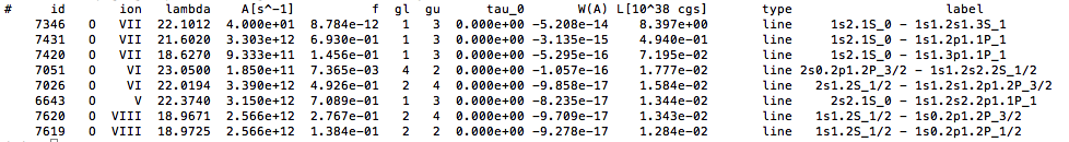
Print a table of information, with the strongest transitions sorted by luminosity.
isis> xstar_page_group( db, strongest; sort="luminosity" );
Plot the model and label the strongest transitions.
 isis> plot_bin_density;

        isis> xlabel( latex2pg( "Wavelength [\\A]" ) );

        isis> ylabel( latex2pg( "Flux [phot/cm^2/s/A]" ) );

        isis> yrange(1.e-13, 1); ylog;

        isis> xrange(18, 24);

        isis> hplot( x1, x2, y, 1 );

        isis> lstyle = line_label_default_style();

        isis> lstyle.top_frac = 0.85;

        isis> lstyle.bottom_frac = 0.7;

        isis> xstar_plot_group( db, strongest );
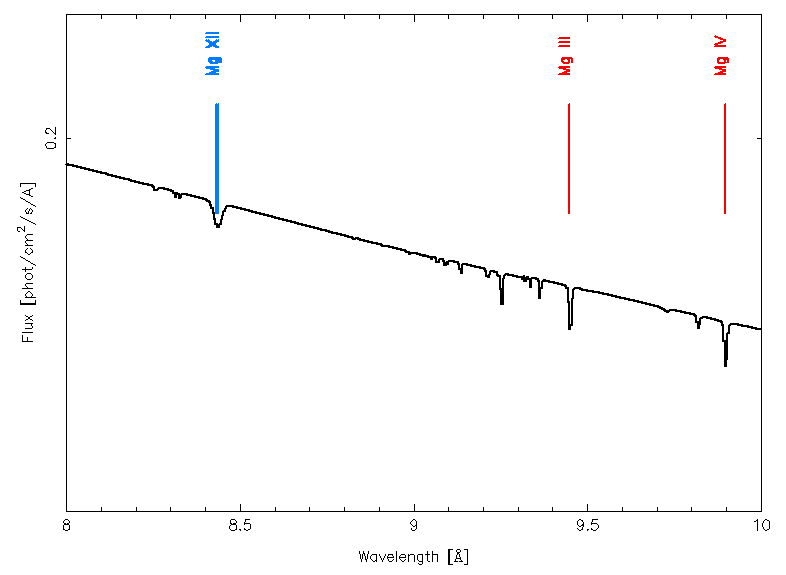
Example 2: Multiple warmabs components
Examine a model of two warm absorbers, offset from eachother in redshift (view script).
 isis> fit_fun( "powerlaw(1) * ( warmabs2(1) + warmabs2(2) )" );

        isis> set_par( "warmabs2(1).Redshift", 0.0 );

        isis> set_par( "warmabs2(2).Redshift", 0.0014 );
Store the redshifts in an array:
isis> z = [ get_par("warmabs2(1).Redshift"), get_par("warmabs2(2).Redshift") ];
Load the files as a merged database:
isis> db_m = xstar_merge( [ "warmabs_1.fits", "warmabs_2.fits" ] );
Find the strongest lines within 8-10 Angstroms. There are some Mg transitions here
that come from both absorption systems.
 isis> s_lines = xstar_strong( 4, db_m; wmin=8.0, wmax=10.0, redshift=z );

        isis> l1 = s_lines[ where(db_m.origin_file[s_lines] == 0) ];

        isis> l2 = s_lines[ where(db_m.origin_file[s_lines] == 1) ];
Plot the two systems using two different colors (2 is red, and 11 is blue):
 isis> xstar_plot_group( db_m, l1, 2, lstyle, z[0] );

        isis> xstar_plot_group( db_m, l2, 11, lstyle, z[1] );
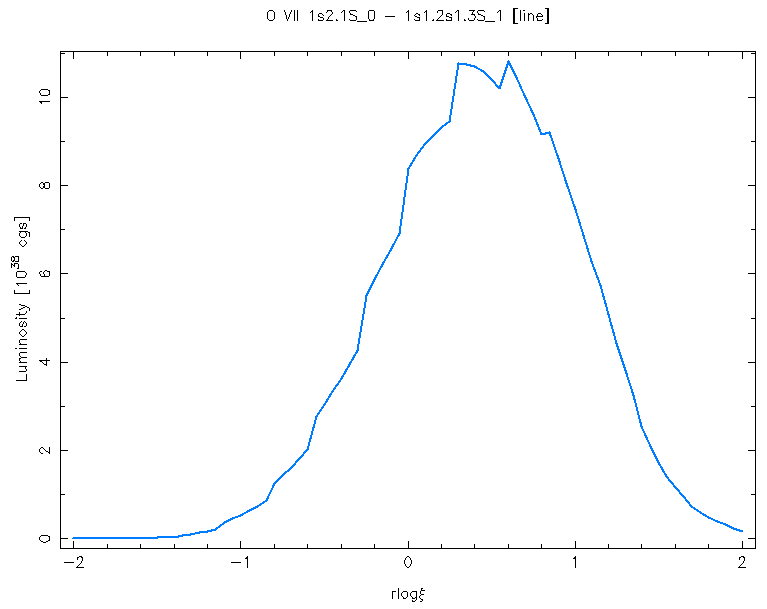
Example 3: A grid of photemis models
See how the forbidden line of the O VII triplet changes in luminosity as a function of ionization parameter, rlogxi (view script).
To run a set of XSTAR models, you need to create two structures:
a wavelength grid:
isis> (x1, x2) = linear_grid( 1.0, 40.0, 10000 );
and a structure containing model information. The built in variable
isis> model_binning = struct{ bin_lo=x1, bin_hi=x2 };_default_model_info is an empty structure with all the necessary
fields. In this example, we set up a photemis model grid over rlogxi = -2 to +2,
using 0.05 spaced sample points.
isis> model_info = @_default_model_info;
(the
isis> set_struct_fields( model_info, "photemis", "rlogxi", -2.0, 2.0, 0.05, model_binning );
@ symbol makes a copy of the variable, instead of a pointer)
Now run the models. This can take awhile.
isis> xstar_run_model_grid( model_info, "/my/rlogxi_example/"; nstart=10 );
Load the models into a gridded database structure:
 isis> fgrid = glob( "/my/rlogxi_example/photemis_*.fits" );

        isis> fgrid = fgrid[ array_sort(fgrid) ];

        isis> pe_grid = xstar_load_tables( fgrid );
Look for the O VII triplet:
 isis> o_vii = where( xstar_el_ion(pe_grid.mdb, O, 7) );

        isis> xstar_page_grid( pe_grid, o_vii );
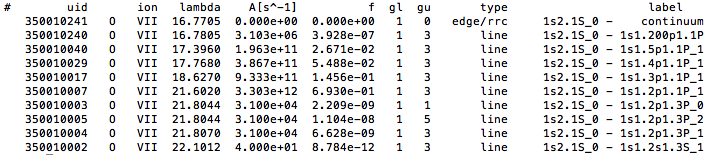
The forbidden line is the last one on the list, at 22.1 Angstroms. The XSTAR output contains
an integer number corresponding to the upper and lower energy level (c.f. the last column
in
xstarlevels.txt). In the case of our O VII triplet, the lower level has an index of 1
and the upper level has an index of 2. To pinpoint this line within the database, use:
isis> o_vii_F = where(xstar_trans( pe_grid.mdb, O, 7, 1, 2 ));
Now we can plot the luminosity of the O VII forbidden line as a function of rlogxi:
 isis> o_vii_F_lum = xstar_line_prop( pe_grid, o_vii_F, "luminosity" );

        isis> rlogxi  = xstar_get_grid_par( pe_grid, "rlogxi" );

        isis> plot( rlogxi, ovii_F_lum, 11 );